Telangana & Andhra Pradesh BIEAP TS AP Intermediate Inter 2nd Year Zoology Study Material Textbook Solutions Guide PDF Free Download, TS AP Inter 2nd Year Zoology Blue Print Weightage 2022-2023, Telugu Academy Intermediate 2nd Year Zoology Textbook Pdf Download, Questions and Answers Solutions in English Medium and Telugu Medium are part of AP Inter 2nd Year Study Material Pdf.
Students can also read AP Inter 2nd Year Botany Syllabus & AP Inter 2nd Year Zoology Important Questions for exam preparation. Students can also go through AP Inter 2nd Year Zoology Notes to understand and remember the concepts easily.
AP Intermediate 2nd Year Zoology Study Material Pdf Download | Sr Inter 2nd Year Zoology Textbook Solutions
- Chapter 1 Human Anatomy and Physiology – I
- Chapter 2 Human Anatomy and Physiology – II
- Chapter 3 Human Anatomy and Physiology – III
- Chapter 4 Human Anatomy and Physiology – IV
- Chapter 5 Human Reproduction
- Chapter 6 Genetics
- Chapter 7 Organic Evolution
- Chapter 8 Applied Biology
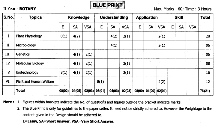
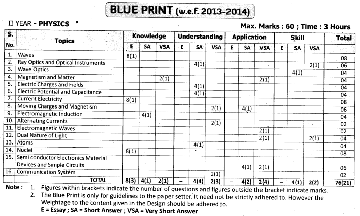
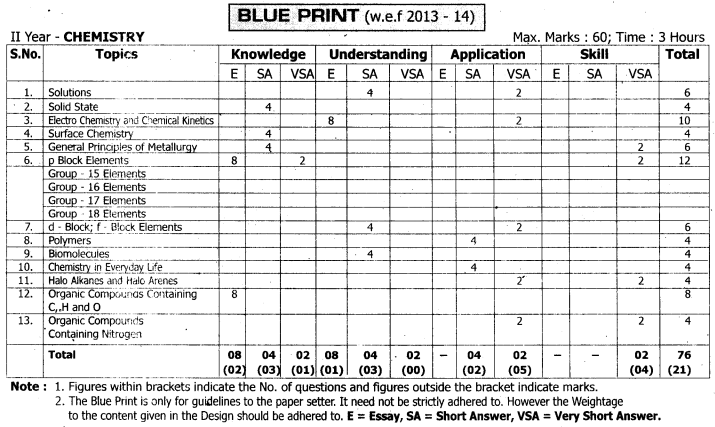
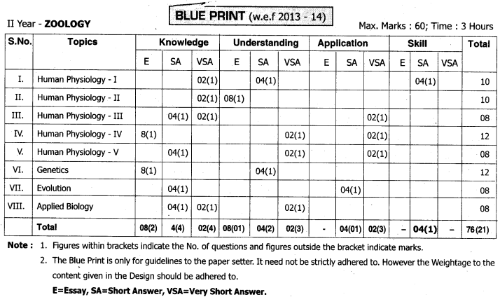
TS AP Inter 2nd Year Zoology Weightage Blue Print 2022-2023
TS AP Inter 2nd Year Zoology Weightage 2022-2023 | TS AP Inter 2nd Year Zoology Blue Print 2022
Intermediate 2nd Year Zoology Syllabus
TS AP Inter 2nd Year Zoology Syllabus
Unit I Human Anatomy and Physiology – I (22 Periods)
Unit IA: Digestion and Absorption
Alimentary canal and digestive glands; Role of digestive enzymes and gastrointestinal hormones; Peri¬stalsis, digestion, absorption, and assimilation of proteins, carbohydrates, and fats, egestion. The calorific value of proteins, carbohydrates, and fats (for box item – not to be evaluated); Nutritional disorders: Protein Energy Malnutrition (PEM), indigestion, constipation, vomiting, jaundice, diarrhea, Kwashiorkor.
Unit IB: Breathing and Respiration
Respiratory organs in animals; Respiratory system in humans; Mechanism of breathing and its regulation in humans – Exchange of gases, transport of gases and regulation of respiration; Respiratory volumes; Respiratory disorders: Asthma, Emphysema, Occupational respiratory disorders – Asbestosis, Silicosis, Siderosis, Black Lung Disease in coal miners.
Unit II Human Anatomy and Physiology – II (22 Periods)
Unit IIA: Body Fluids and Circulation
Covered in I year composition of lymph and functions; Clotting of blood; Human circulatory system- the structure of the human heart and blood vessels; Cardiac cycle, cardiac output, double circulation; regulation of cardiac activity; Disorders of circulatory system: Hypertension, coronary artery disease, angina pectoris, heart failure.
Unit IIB: Excretory Products and their Elimination
Modes of excretion – Ammonotelism, Ureotelism, Uricotelism; Human excretory system – the structure of kidney and nephron; Urine formation, osmoregulation; Regulation of kidney function – Renin – Angiotensin – Aldosterone system, Atrial Natriuretic Factor, ADH and diabetes insipidus; Role of other organs in excretion; Disorders: Uraemia, renal failure, renal calculi, nephritis, dialysis using artificial kidney.
Unit III Human Anatomy and Physiology – III (20 Periods)
Unit IIIA: Muscular and Skeletal System
Skeletal muscle – ultrastructure; Contractile proteins & muscle contraction; Skeletal system and its functions; Joints, (to be dealt with relevance to practical syllabus); Disorders of the muscular and skeletal system: myasthenia gravis, tetany, muscular dystrophy, arthritis, osteoporosis, gout, Gregor Mortis.
Unit IIIB: Neural Control and Co-ordination
The nervous system in human beings – Centralnfervous system. Peripheral nervous system and Visceral nervous system; Generation and conduction of nerve impulse; Reflex action: Sensory perception; Sense organs; Brief description of other receptors; Elementary structure and functioning of eye and ear.
Unit IV Human Anatomy and Physiology – IV (15 Periods)
Unit IVA: Endocrine System and Chemical Co-ordination
Endocrine glands and hormones; Human endocrine system – Hypothalamus, Pituitary, Pineal, Thyroid, Parathyroid, Adrenal, Pancreas; Gonads; Mechanism of hormone action (Elementary idea only); Role of hormones as messengers and regulators) Hypo and Hyperactivity and related disorders: Common disorders – Dwarfism, acromegaly, cretinism, goiter, exophthalmic goiter, diabetes, Addison’s disease, Cushing’s syndrome. (Diseases & disorders to be dealt in brief).
Unit IVB: Immune System
Basic concepts of Immunology – Types of Immunity – Innate Immunity, Acquired Immunity, Active and Passive Immunity, Cell-mediated Immunity and Humoral Immunity, Interferon, HIV, and AIDS.
Unit V Human Reproduction (22 Periods)
Unit VA: Human Reproductive System
Male and female reproductive systems; Microscopic anatomy of testis & ovary; Gametogenesis is Sper-matogenesis & Oogenesis; Menstrual cycle; Fertilization, Embryo development up to blastocyst formation. Implantation; Pregnancy, placenta formation. Parturition, Lactation (elementary idea).
Unit VB: Reproductive Health
Need for reproductive health and prevention of sexually transmitted diseases (STD); Birth control – need and methods, contraception and medical termination of pregnancy (MTP); Amniocentesis; infertility and assisted reproductive technologies – IVF-ET, ZIFT, GIFT (Elementary idea for general awareness).
Unit VI Genetics (20 Periods)
Heredity and variation: Mendel’s laws of inheritance with reference to Drosophila. (Drosophila melanogaster Grey, Black body colour; Long, Vestigial wings), Pleiotropy; Multiple alleles: Inheritance of blood groups and Rh-factor; Co-dominance (Blood groups as an example); Elementary idea of polygenic inher¬itance: Skin colour in humans (refer Sinnott, Dtinn and Dobzhansky); Sex determination – in humans, birds, Fumea moth, genic balance theory of sex determination in Drosophila melanogaster and honey bees; Sex-linked inheritance – Haemophilia, Colour blindness; Mendelian disorders in humans: Thalassemia, Haemophilia, Sickle celled anemia, cystic fibrosis PKU, Alkaptonuria; Chromosomal disorders – Down’s syndrome. Turner’s syndrome and Klinefelter syndrome; Genome, Human Genome Project and DNA Finger Printing.
Unit VII Organic Evolution (15 Periods)
Origin of Life, Biological evolution and Evidence for biological evolution (palaeontological, comparative anatomical, embryological and molecular evidence); Theories of evolution: Lamarckism (in brief), Darwin’s theory of Evolution – Natural Selection with example (Kettlewell’s experiments on Biston Bulgaria). Mutation Theory of Hugo De Vries; Modern synthetic theory of Evolution – Hardy- Weinberg law; Types of Natural Selection; Geneflow and genetic drift; Variations (mutations and genetic recombination); Adaptive radiation – viz., Darwin’s finches and adaptive radiation in marsupials; Human evolution; Speciation – Allopatric, sym- Patric; Reproductive isolation.
Unit VIII Applied Biology (15 Periods)
Apiculture; Animal Husbandry:’Pisciculture, Poultry management. Dairy management; Animal breeding; Bio-medical Technology: Diagnostic Imaging (X-Ray, CT scan, MRI), ECG, EEG; Application of Biotechnology in health: Human insulin and vaccine production; Gene Therapy; Transgenic Animals; ELISA; Vaccines, MABs, Cancer biology, stem cells.
We hope that this Telangana & Andhra Pradesh BIEAP TS AP Intermediate Inter 2nd Year Zoology Study Material Textbook Solutions Guide PDF Free Download 2022-2023 in English Medium and Telugu Medium helps the student to come out successful with flying colors in this examination. This Sr Inter 2nd Year Zoology Study Material will help students to gain the right knowledge to tackle any type of questions that can be asked during the exams.