Students can go through Telangana & Andhra Pradesh BIEAP TS AP Inter 1st Year Physics Notes Pdf Download in English Medium and Telugu Medium to understand and remember the concepts easily. Besides, with our AP Jr Inter 1st Year Physics Notes students can have a complete revision of the subject effectively while focusing on the important chapters and topics.
Students can also go through AP Inter 1st Year Physics Study Material and AP Inter 1st Year Physics Important Questions for exam preparation.
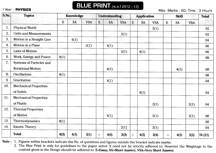
AP Intermediate 1st Year Physics Notes
- Chapter 1 Physical World Notes
- Chapter 2 Units and Measurements Notes
- Chapter 3 Motion in a Straight Line Notes
- Chapter 4 Motion in a Plane Notes
- Chapter 5 Laws of Motion Notes
- Chapter 6 Work, Energy and Power Notes
- Chapter 7 Systems of Particles and Rotational Motion Notes
- Chapter 8 Oscillations Notes
- Chapter 9 Gravitation Notes
- Chapter 10 Mechanical Properties of Solids Notes
- Chapter 11 Mechanical Properties of Fluids Notes
- Chapter 12 Thermal Properties of Matter Notes
- Chapter 13 Thermodynamics Notes
- Chapter 14 Kinetic Theory Notes
These TS AP Intermediate 1st Year Physics Notes provide an extra edge and help students to boost their self-confidence before appearing for their final examinations. These Inter 1st Year Physics Notes will enable students to study smartly and get a clear idea about each and every concept discussed in their syllabus.