AP Board 8th Class Maths Solutions Chapter 7 Frequency Distribution Tables and Graphs Ex 7.3

AP State Syllabus AP Board 8th Class Maths Solutions Chapter 7 Frequency Distribution Tables and Graphs Ex 7.3 Textbook Questions and Answers.

AP State Syllabus 8th Class Maths Solutions 7th Lesson Frequency Distribution Tables and Graphs Exercise 7.3

Question 1.
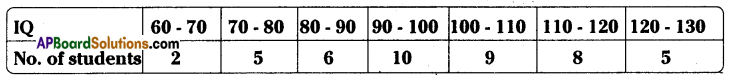
The following table gives the distribution of45 students across the different levels of intelligent Quotient. Draw the histogram for the data.

Solution:

Steps of construction:
1. Calculate the difference between mid values of two consecutive classes
∴ h = 75 – 65 = 10
∴ Class interval (C.I) = 10

2. Select such a right scale
on X-axis 1 cm = 10 units
on Y-axis 1 cm 1 student

3. Construct a histogram with C.Is as width and frequencies as lengths.

Question 2.
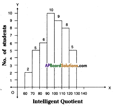
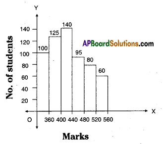
Construct a histogram for the marks obtained by 600 students in the VII class annual
examinations.

Solution:
Classes will be prepared on class marks.
Step – 1: Take the difference between the mid values of two consecutive classes.
∴ h = 400 – 360 = 40

Step – 2: Let the lower and upper boundaries be taken as x – \(\frac{h}{2}\) , x + \(\frac{h}{2}\)
∴ x – \(\frac{h}{2}\) = 360 – \(\frac{40}{2}\) = 360 – 20 = 340
x + \(\frac{h}{2}\) = 360 + \(\frac{40}{2}\) = 360 + 20 = 380

Step – 3 : Select the scale
on X-axis 1 cm = 1 C.I (mid values)
on Y-axis 1 cm = 20 students

Step – 4 : Take C.I’s as width, frequencies as lengths.
Then construct the histogram.

Class Marks	Class Interval	Frequency
360	340- 380	100
400	380- 420	125
440	420-460	140
480	460-500	95
520	500-540	80
560	540-580	60

Scale : On Y – axis no. of students = 20, On X – axis take marks of students.

Question 3.
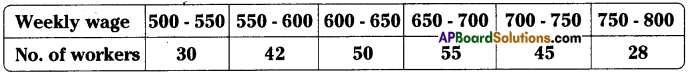
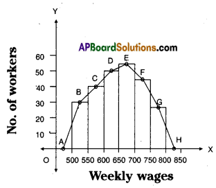
Weekly wages of 250 workers in a factory are given in the following table. Construct the histogram and frequency polygon on the same graph for the data given.
using the histogram. (Use separate graph sheets)

Solution:

Class Interval (Weekly wages)	Frequency (No. of workers)	Mid values
500-550	30	525
550-600	42	575
600-650	50	625
650-700	55	675
700-750	45	725
750 -800	28	775
	N = 250

Steps of constructIon:

1. C.I. = Difference of two consecutive mid values = h = 575 – 525 = 50
2. Scale : On X-axis 1 cm = ₹ 50
   On Y-axis 1 cm = lo members
3. Take on X-axis width of C.I, on Y-axis frequncies.
4. Keep points A, B, C, D, E, F, G, H on the mid points of rectangles.
5. The area of a histogram is equal to the area of a polygon.

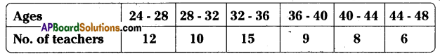
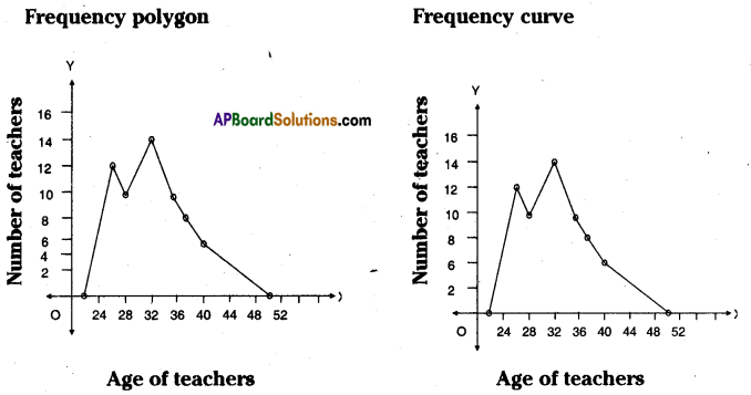
Question 4.
Ages of 60 teachers in primary schools of a Mandai are given in the following frequency distribution table. Construct the Frequency polygon and frequency curve for the data without using the histogram. (Use separate graph sheets)

Solution:
Construction of frequency polygon:

1. Class interval = The difference between two mid values of classes
   = 30 – 26 = 4
2. Scale : On X-axis take the age of teachers
   On Y-axis take number of teachers.
3. Scale: On X-axis 1 cm = 4units
   On Y- axis 1 cm = 2 units
4. Take the widths of classes on X – axis. Frequencies on Y – axis.
5. The points are formed on the graph sheet are joined by a scale then the required frequency polygon and if the points are joined by hand frequency curve will be formed.

Question 5.
Construct class intervals and frequencies for the foliowing distribution tabie. Also draw the ogive curves for the same.

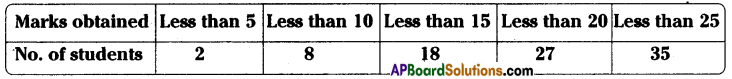
Solution:
Steps of constructIon:
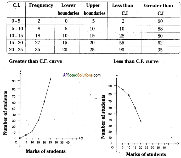
Step – 1: If the given frequency distribution is in inclusive form, then convert it into an
exclusive form.

Step – 2: Calculate the less than cumulative frequency.

Step – 3: Mark the upper boundaries of the class intervals along X-axis and their corresponding cumulative frequencies along Y-axis.

Select the scale:
X – axis 1 cm = 1 class interval
Y – axis 1 cm = 10 students

Step – 4: Also, plot the lower boundary of the first class (upper boundary of the class previous to first class) interval with cumulative frequency 0.

Step – 5: Join these points by a free hand curve to obtain the required ogive.
Similarly we can construct ‘greater than cumulative frequency curve by taking greater than cumulative on Y – axis and corresponding ‘lower boundaries’ on the
X-axis.